This post will be covering the two models that were set up in TensorFlow to process MNIST digit data, how training was conducted and finally how the results were converted into a tangible model to be leveraged down stream. This post is part of the TensorFlow + Docker MNIST Classifier series.
I will not be covering the basics of TensorFlow in these posts. Typically I am not a huge fan of programming literature myself with the massive amount of resources available online, however for learning TensorFlow I highly recommend this e-book for grasping the fundamentals.
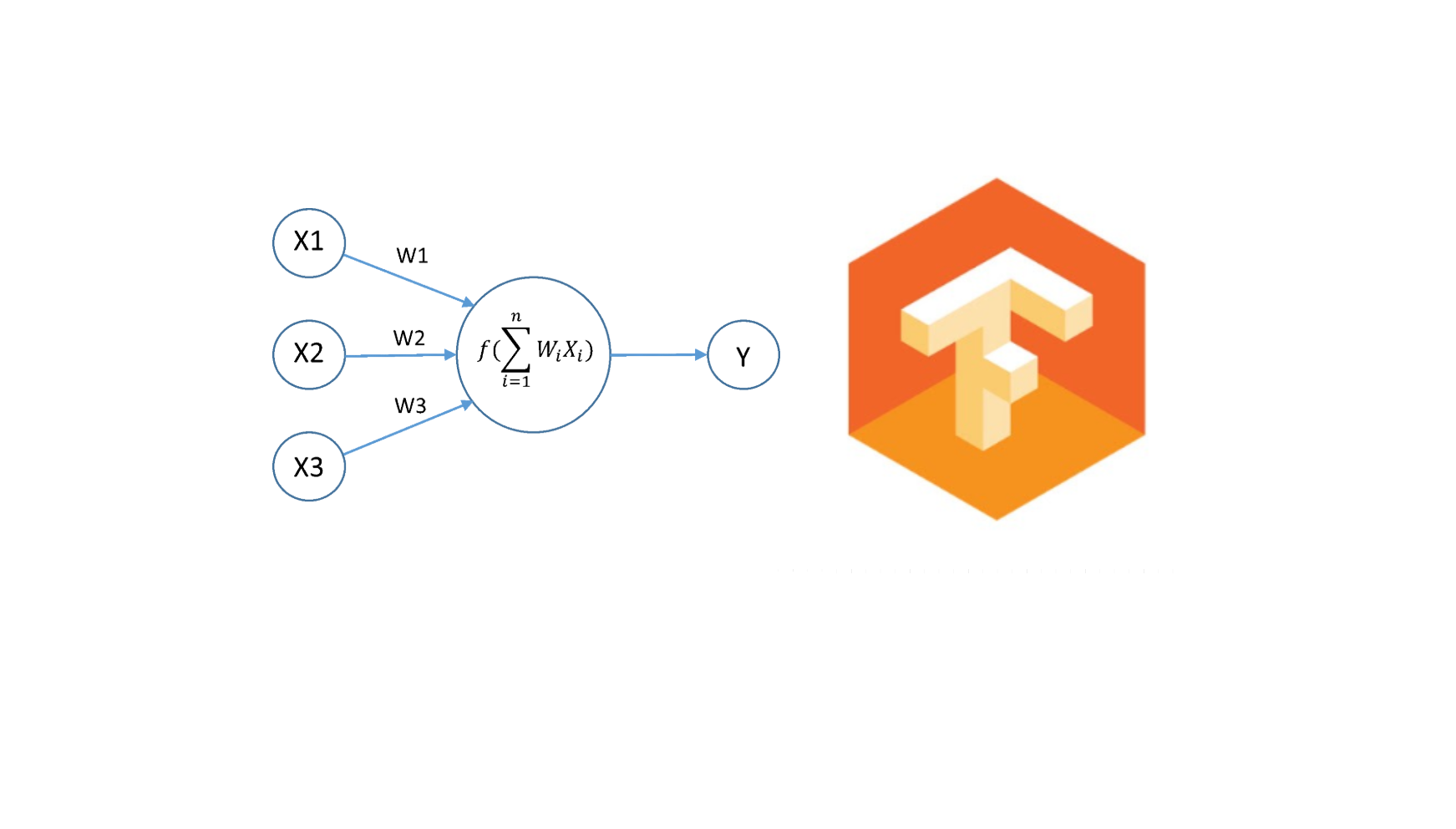
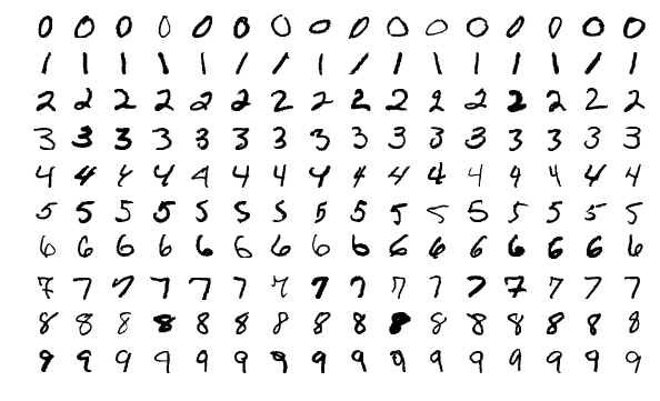
The Data Set (MNIST): This is one of the most popular machine learning data sets on the internet at the moment. It consists of tens of thousands of 28 x 28 labeled hand written written digits like the one below.
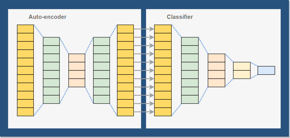
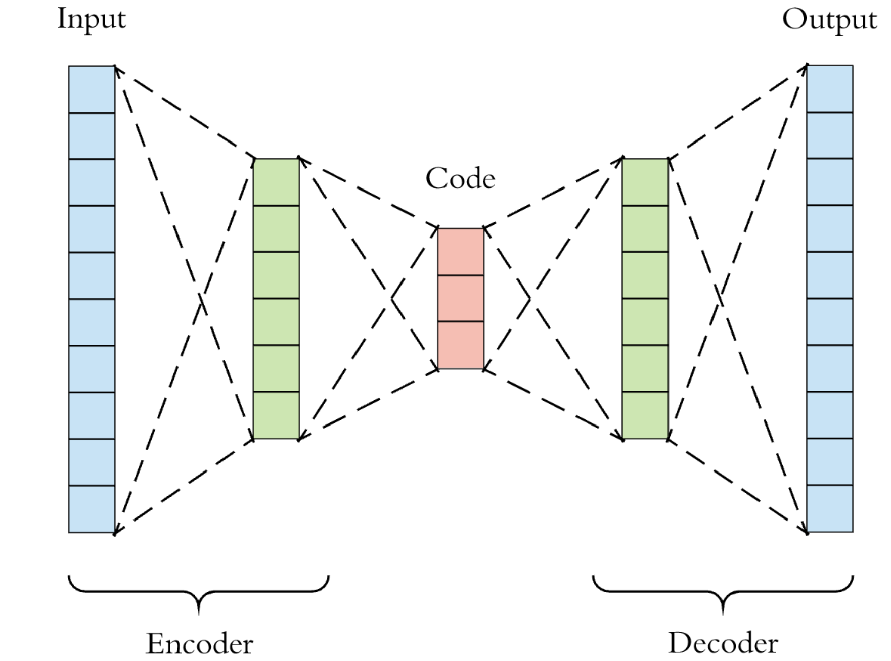
One of the key success criteria for this project was the use of multiple models in the final solution. The first model will be an auto-encoder to standardize the image data and the second model will classify it.
Features and targets
The features or digits will be passed through the model as a 784 dimensional vectors with each element of the vector representing pixel intensity (white to black) of each pixel in the 28 x 28 image. Scaling was used on the feature data to improve performance converting the value range from [0.0, 255.0] to [0.0, 1.0] by dividing each value by 255.
Data set labels (targets) are a single dimensional vector with values ranging from 0 - 9, representing the 10 potential digit classes. In order to improve model performance and simplicity these were transformed into a 10 dimensional one-hot representation with each dimension representing the probability of the associated digit e.g. [5] -> [0, 0, 0, 0, 0, 1, 0, 0, 0, 0].
The model
One of the goals of this project was to implement a system with 2 models and I chose to use an auto-encoder as my first model and a basic classifier for my second as illustrate below.
Keras is used to simplify development and training, config files are used to store hyperparameters and file paths and I developer a basic helper for loading MNIST image data as I am not using Keras for data loading.
| Supporting python objects | Description |
|---|---|
| Config | Configuration file for the training |
| MNISTProcessor | MNIST data loader |
| DataWrapper | Object to handle training and testing data |
| Visualizer | Stored functions to help visualize results |
The Auto-encoder: There is a lot of great material on the auto-encoder network online including the wiki entry here. In a nutshell an auto-encoder is an unsupervised symmetrical neural network that compresses the feature vector into significantly fewer dimensions. The network is trained by using features as both the input and output of the network, teaching the filters to compress the features. One of the key uses of the auto-encoder is noise reduction and this is what it will be used for here.
| Parameters | |
|---|---|
| Graph | 728-152-76-38-4-38-76-152-728 |
| Activation | Tanh for all layers |
| Loss Function | Mean squared error |
| Optimizer | Adadelta initial learning rate 1.0 |
| Batch Size | 50 |
| Epochs | 500 |
Using Keras we can implement the neural network using the following code.
from tensorflow.keras.layers import Input, Dense
from tensorflow.keras.models import Model
from tensorflow.keras.callbacks import ModelCheckpoint
from tensorflow.compat.v1 import flags
from tensorflow.keras import optimizers
import sys, os
import config as conf

#set up and parse custom flags
flags.DEFINE_integer('model_version', conf.version, "Width of the image")
flags.DEFINE_boolean('rebuild', False, "Drop the checkpoint weights and rebuild model     from scratch")
flags.DEFINE_string('lib_folder', conf.lib_folder, "Local library folder")
FLAGS = flags.FLAGS

#mount the library folder
sys.path.append(os.path.abspath(FLAGS.lib_folder))
from data import MNISTProcessor
import visualizer as v

#load data
data_processor = MNISTProcessor(conf.data_path, conf.train_labels,
                            conf.train_images, '', '')
x_data_train, y_data_train = data_processor.load_train(normalize=True).get_training_data()

#initialize the network
input_layer = Input(shape=(784,), name='input')
network = Dense(152, activation='tanh', name='dense_1')(input_layer)
network = Dense(76, activation='tanh', name='dense_2')(network)
network = Dense(38, activation='tanh', name='dense_3')(network)
network = Dense(4, activation='tanh', name='dense_4')(network)
network = Dense(38, activation='tanh', name='dense_5')(network)
network = Dense(76, activation='tanh', name='dense_6')(network)
network = Dense(152, activation='tanh', name='dense_7')(network)
output = Dense(784, activation='tanh', name='output')(network)

autoencoder = Model(inputs=input_layer, outputs=output, name='autoencoder')
autoencoder.compile(optimizer=optimizers.Adadelta(learning_rate=1.0), loss='MSE',     metrics=['accuracy'])

# Create a callback that saves the model's weights
cp_callback = ModelCheckpoint(filepath=conf.checkpoint_path, save_weights_only=True, verbose=1)

#load an existing model to continue training
if(not FLAGS.rebuild):
    try:
        autoencoder.load_weights(conf.checkpoint_path)
    except:
        print('No checkpoint found, building filters from scratch.')

#run the training
autoencoder.fit(x_data_train, x_data_train,
            epochs=conf.epochs,
            batch_size=conf.batch_size,
            shuffle=True,
            callbacks=[cp_callback])

#save the production version of the model
try:
    os.mkdir(conf.final_model_path + '/' + str(FLAGS.model_version))
except OSError:
    print ("Creation of the directory %s failed" % conf.final_model_path + '/' +     str(FLAGS.model_version))

autoencoder.save(conf.final_model_path + '/' + str(FLAGS.model_version),     overwrite=True, save_format='tf')

autoencoder.summary()

# run a sample for visualization
clean_images = autoencoder.predict(x_data_train)
v.visualize_autoencoding(x_data_train, clean_images, digits_to_show=10)
To break down the code a little
lines 10-13 - using tensorflow flags to pull command line argument values
lines 21-23 - process the MNIST data set into features and labels
lines 26-37 - set up the neural network strcture and optimizer
lines 40 - set up callback for saving checkpoints during training
lines 43-47 - load any existing checkpoints
lines 50-54 - train the model
lines 57-62 - save a production version that will be ready for serving
lines 64-68 - display final model strcture and some sample autoencodings
The following function was created to help visualize the auto-encoder result.
import matplotlib.pyplot as plt


def visualize_autoencoding(original_data, decoded_data, digits_to_show=10):
    plt.figure(figsize=(20, 4))
    for i in range(digits_to_show):
        # display original
        sub_plot = plt.subplot(2, digits_to_show, i + 1)
        plt.imshow(original_data[i].reshape(28, 28))
        plt.gray()
        sub_plot.get_xaxis().set_visible(False)
        sub_plot.get_yaxis().set_visible(False)

        # display reconstruction
        sub_plot = plt.subplot(2, digits_to_show, i + 1 + digits_to_show)
        plt.imshow(decoded_data[i].reshape(28, 28))
        plt.gray()
        sub_plot.get_xaxis().set_visible(False)
        sub_plot.get_yaxis().set_visible(False)
    plt.show()
this function can be called like so: visualize_autoencoding(x_data_train, clean_images, digits_to_show=4) from our training program after the training is completed.
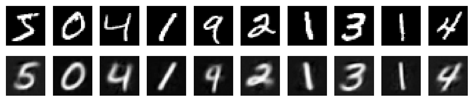
After training my error loss was around 0.025 and you can see below what a few sample images looked like after being passed through the trained auto-encoder. The result could be improved but this should be satisfactory for our needs.
The Classifier: The second model will take the 784 dimensional vector output by the auto-encoder and and classifying the data into one of the 10 possible digit values [0, 9]. A simple tanh activated deep neural network will be used.
| Parameters | |
|---|---|
| Graph | 784-140-80-40-10 |
| Activation | Tanh for all layers |
| Loss Function | Mean squared error |
| Optimizer | Adadelta initial learning rate 1.0 |
| Batch Size | 50 |
| Epochs | 100 |
Keras was used to implement the classifier as well. We first load and process the image data through the auto-encoder before using as the feature input for training of the classifier.
from tensorflow.keras.layers import Input, Dense
from tensorflow.keras.models import Model
from tensorflow.keras import optimizers
from tensorflow.compat.v1 import flags
import tensorflow.keras as Keras
from tensorflow.keras.callbacks import ModelCheckpoint
import sys, os
import config as conf

#set up and parse custom flags
flags.DEFINE_integer('model_version', conf.version, "Width of the image")
flags.DEFINE_boolean('rebuild', False, "Drop the checkpoint weights and rebuild model from scratch")
flags.DEFINE_string('lib_folder', conf.lib_folder, "Local library folder")
flags.DEFINE_integer('encoder_version', 1, "Autoencoder version to use")
FLAGS = flags.FLAGS

#mount the library folder
sys.path.append(os.path.abspath(FLAGS.lib_folder))
from data import MNISTProcessor

#load data
data_processor = MNISTProcessor(conf.data_path, conf.train_labels,
                            conf.train_images, '', '')
x_data_train, y_data_train = data_processor.load_train(normalize=True).get_training_data()

# Load the autoencoder model, including its weights and then process images
autoencoder = Keras.models.load_model(conf.autoencoder_model_path + '/' +  str(FLAGS.encoder_version))
clean_images = autoencoder.predict(x_data_train)

#initialize the classification network
input_layer = Input(shape=(784,))
network = Dense(140, activation='tanh', name='dense_1')(input_layer)
network = Dense(80, activation='tanh', name='dense_2')(network)
network = Dense(40, activation='tanh', name='dense_3')(network)
output = Dense(10, activation='tanh', name='dense_4')(network)

classifier = Model(inputs=input_layer, outputs=output, name='classifier')
classifier.compile(optimizer=optimizers.Adadelta(learning_rate=1.0), loss='MSE', metrics=['accuracy'])

# Create a callback that saves the model's weights
cp_callback = ModelCheckpoint(filepath=conf.checkpoint_path, save_weights_only=True, verbose=1)

#load an existing model to continue training
if(not FLAGS.rebuild):
    try:
        classifier.load_weights(conf.checkpoint_path)
    except:
        print('No checkpoint found, building filters from scratch.')

#run the model
classifier.fit(clean_images, y_data_train,
            epochs=conf.epochs,
            batch_size=conf.batch_size,
            shuffle=True,
            callbacks=[cp_callback])

#save the production version of the model
try:
    os.mkdir(conf.final_model_path + '/' + str(FLAGS.model_version))
except OSError:
    print ("Creation of the directory %s failed" % conf.final_model_path + '/' + str(FLAGS.model_version))

classifier.save(conf.final_model_path + '/' + str(FLAGS.model_version), overwrite=True, save_format='tf')

classifier.summary()
To break down the code a little
lines 11-15 - using tensorflow flags to pull command line argument values
lines 22-24 - process the MNIST data set into features and labels
lines 27-28 - load the autoencoder model and process the feature data set
lines 31-38 - set up the neural network strcture and optimizer
lines 41 - set up callback for saving checkpoints during training
lines 45-49 - load any existing checkpoints
lines 51-55 - train the model
lines 57-62 - save a production version that will be ready for serving
lines 65 - display final model strcture
Lessons learned
Poor initial model convergence - I wrote my initial code using the stand alone keras library, however due to challenges of saving the models in a servable format I had to switch the the tf.keras library instead. After my switch my models flat out refused to converge during training. After many hours of debugging I discovered that the keras.optimizers.Adadelta optimizer uses a default starting learning rate of 1.0, where as the tf.keras.optimizersAdadelta optimizer initializes with a learning rate of 0.001. Forcing the learning rate addressed this issue for me and you can see this reflected in my code.
For the lazy
My results can be reproduced with the following commands:
#navigate to where you would like to generate the repository
$ git clone https://github.com/adidinchuk/tf-mnist-project
$ cd tf-mnist-project

$ curl http://yann.lecun.com/exdb/mnist/train-images-idx3-ubyte.gz --output data/train-images-idx3-ubyte.gz
$ curl http://yann.lecun.com/exdb/mnist/train-labels-idx1-ubyte.gz --output data/train-labels-idx1-ubyte.gz

#Unzip the data using your prefer compression tool.
#Make sure the file names and location do not change,
#otherwise you will have to make the appropriate changes in the config filesv

#once the data has been extracted train the autoencoder model using
$ py -3.6 src/autoencoder/graph.py --model_version 1

#after the training completes you should see a .pb model file in the models/autoencoder/production folder

#now run the classifier training
$ py -3.6 src/classifier/graph.py  --model_version 1 --encoder_version 1

#after the training completes you should see a .pb model file in the models/classifier/production/#/ folder
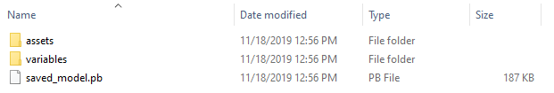
You should now see the production models under models/autoencoder/production/1 and models/classifier/production/1 that looks like this:
The entire TensorFlow github repository along with complete instructions on running the model can be found here. Now that we have both the auto-encoder and classifier models generated we can take a look at deploying them via TensorFlow serving, which I will do in my next post.
Here is a summary of the components involved in this project:
| Section | Git Repository |
|---|---|
| Introduction | N/A |
| The Models | tf-mnist-project |
| Serving Models | tf-serving-mnist-project |
| The User Interface | angular-mnist-project |